14 Combined Loads
Introduction
Click to expand
In this chapter, we will use of all of the previously discussed methods to determine normal and shear stress resulting from axial forces (Chapter 5), bending moments (Chapter 9), pressure (Chapter 13), transverse loads (Chapter 10), and torsion (Chapter 6) to determine an overall general stress state for any given point on a structure.
In Section 14.1, the various sources of normal stress are reviewed and expanded on. They will be reframed in terms of general axes so as to clarify which other stresses they may combine with. In Section 14.1.1 we will revisit bending stress to express the unsymmetric bending stress equation in terms of general cross-sectional axes (recall in Chapter 9, the cross-sectional axes were always y and z). In Section 14.1.2, eccentric loading, which is a specific instance of combined normal stress in which normal forces result in bending, will be considered.
In Section 14.2, we will focus on combining the various sources of shear stress to determine the total shear stress. To expand on the concepts discussed and used in Chapter 6 and Chapter 10, we will perform calculations based on both possible transverse loading directions as well as torsion. As in Section 14.1, this will be done with a general set of coordinate axes.
In Section 14.3, we will further expand the above cases to situations in which all combinations of loading are possible and the general stress state is determined.
Note that the determination of the internal reactions for the general problems presented in this chapter will require the use of 3D equilibrium equations, particularly for determining bending moments and torsion. You may find it helpful to review Section 1.3 to understand these calculations.
14.1 Combined Normal Stress
Click to expand
All forms of normal stress previously discussed act in the longitudinal (also referred to as axial) direction except for the hoop stress from pressure. The longitudinal direction is the direction normal to the cross-sectional location of the point for which stress is being evaluated.
To be able to discuss directions and stress components in general terms, we will consider the loadings and stresses in terms of the longitudinal direction (L) at the point in the structure being considered, the centroidal vertical axis of the cross-section (V), and the centroidal horizontal axis of the cross-section (H). The specific axes that these terms refer to depends on how the axes are specified generally for a structure as well as the location of the point in question.
For example, consider the structure in Figure 14.1 with the x, y, z axes oriented at the origin as shown. For point P on the structure, the longitudinal axis is the x-axis and the vertical and horizontal axes of the cross-section are the y-axis and z-axis, respectively. On the other hand, for point Q, the longitudinal axis is the y-axis and the vertical and horizontal axes of the cross-section are the z-axis and x-axis, respectively.
We have seen that axial load, bending moments, and pressure all result in normal stresses. We can express the 2D normal stress state for any given point as:
\[ \sigma_L=\frac{\sum F_L}{A}+\sigma_{bending}+\frac{p r}{2 t} \]
in the longitudinal direction and:
\[ \sigma_{hoop}=\frac{p r}{t} \]
in the direction of the other planar axis of the point in question. For the example given in Figure 14.1, both points are in the x-y plane, but the hoop direction is the y direction for point P and the x direction for point Q.
In the above stress equation, FL is the total force in the direction normal to the cross-section (same direction as the longitudinal direction). It is positive if the total normal force is tensile and negative if compressive. In addition, A is the cross-sectional area, p is the internal pressure, r is the inside radius of a pipe, and t is the wall thickness of a pipe. The pressure term will always be positive for internal pressure. Of course, for a solid cross-section, or a hollow cross-section with no pressure, the hoop stress and the last term of the longitudinal stress would be 0.
To help break down this analysis, Section 14.1.1 presents further clarification on finding bending stress for general coordinate axes. Section 14.1.2 discusses the specific combined loading case of an axial force that also results in bending.
14.1.1 Generalized Bending Stress Equation
In Section 9.1 , an equation for bending stress based on having bending around the cross-sectional axes of y and z was derived. That equation is:
\[ \sigma_x=-\frac{M_z y}{I_z}+\frac{M_y z}{I_y} \]
The negative sign in front of the Mz expression and the plus in front of the My expression are specifically related to the y and z cross-sectional axes as oriented as they were in Chapter 9, with the z-axis positive horizontally to the left and the y axis positive vertically upwards. However, because cross-sectional axes for any given point on a structure can vary based on both how the global axes are specified and on the location of the point within the structure, we will need to know how to apply the bending stress equation for a general set of axes before we can combine this stress with other sources of normal stress.
In any given loading situation, the bending moments are the moments around the cross-sectional centroidal axes. If the cross-sectional centroidal axes are thought of generally as the vertical axis (V) and the horizontal axis (H) as shown in Figure 14.2, the resulting stress would be in the longitudinal direction (L), and we can express the unsymmetric bending stress equation as:
\[ \boxed{\sigma_{L(bending})= \pm\left|\frac{M_V d_H}{I_V}\right| \pm\left|\frac{M_H d_V}{I_H}\right|} \tag{14.1}\]
𝜎𝐿 = Bending stress in the longitudinal direction [Pa, psi]
MV = Bending moment around the vertical axis [N⸱m, lb⸱in.]
MH = Bending moment around the horizontal axis [N⸱m, lb⸱in.]
dH = Horizontal distance between the point on the cross-section for which the stress is being calculated and the V axis [m, in.]
dV = Vertical distance between the point on the cross-section for which the stress is being calculated and the H axis [m, in.]
IV = the moment of inertia about the vertical axis [m4, in.4]
IH = Area moment of inertia about the horizontal axis [m4, in.4]
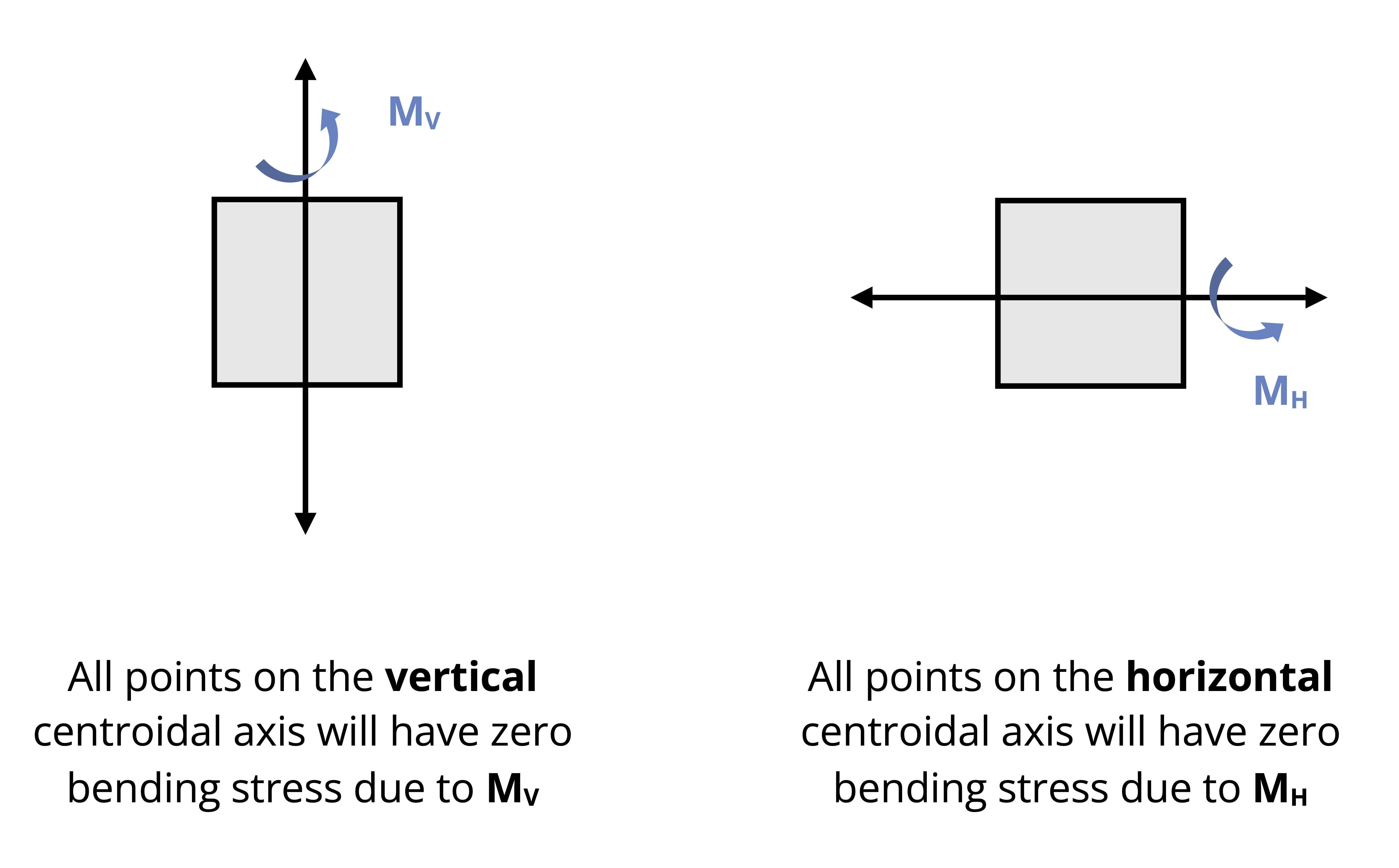
The sign on each individual term needs to be determined by inspection of the bending direction. The side of the cross section that would be on the “inside” of the bend will be in compression and vice versa. Figure 14.3 illustrates the sense of the bending moment around the horizontal axis that would result in compression above the H axis and tension below. Figure 14.4 illustrates the sense of bending moment around the vertical axis that would result in tension to the left of the V axis and compression to the right. The bending moment is shown for a section above and below a cut on a vertical structure and to the left and right of a cut on a horizontally oriented structure. The opposite directions of bending moment would lead to the opposite signs of stress.
If visualization is difficult, one can use the following tool:
- Draw the applied moment arrows around the V and H axes on the cross-section in the correct sense. Make sure to draw them such that they go over (or in front of) the bending axis (as opposed to under or behind)
- The side (top/bottom for moments around the H axis and left/right for the moments around the V axis) the arrows point into are the compressive sides and the sides the tails of the arrows are on are the tensile sides.
The use of this tool will be demonstrated for the bending stress calculation in Example 14.1.
It will also be helpful to note that the bending stress for a point that lies directly on a centroidal axis will be zero for bending around that axis since the bending axis is the neutral axis for that direction of bending, as shown in Figure 14.5.
Example 14.1
The internal bending moments on a 32 mm diameter solid steel rod are found to be Mx = 376 kN mm and Mz = 204 kN mm as shown. Determine the bending stress at points P and Q.
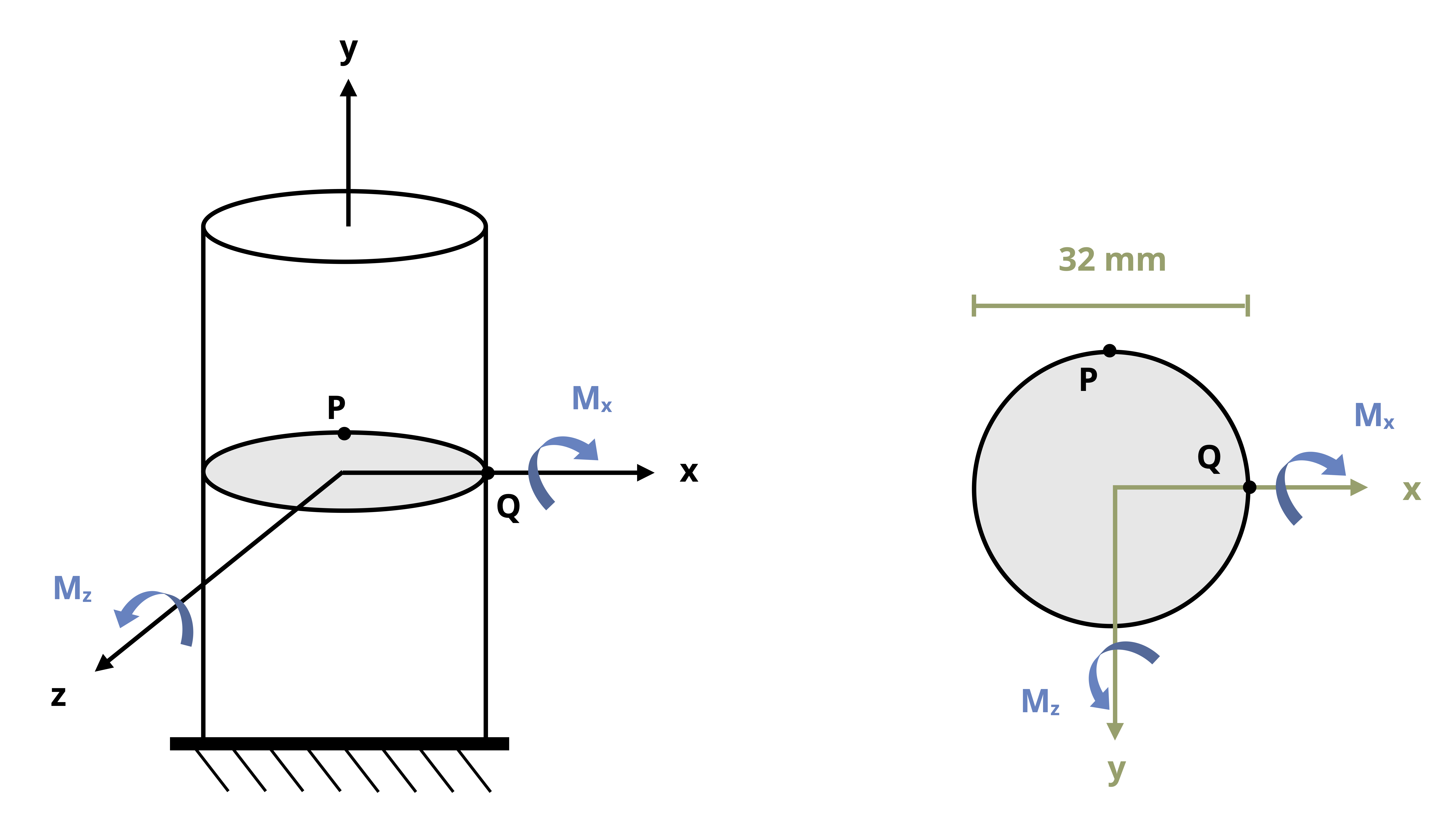
Drawing the cross-section, we can see that the vertical axis of the cross section is the z-axis and the horizontal axis of the cross section is the x-axis. The resulting stress is in the longitudinal direction, which is the y-axis. The bending stress equation can then be expressed as:
\[ \sigma_y= \pm\left|\frac{M_z x}{I_z}\right| \pm\left|\frac{M_x z}{I_x}\right| \]
The magnitudes of the bending moments are given. With the circular cross-section, the moment of inertia of both cross-sectional axes are:
\[ I_x=I_y=\frac{\pi}{4} r^4=\frac{\pi}{4}(16{~mm})^4=51.47 \times 10^3{~mm}^4=51.47 \times 10^{-9}{~m}^4 \]
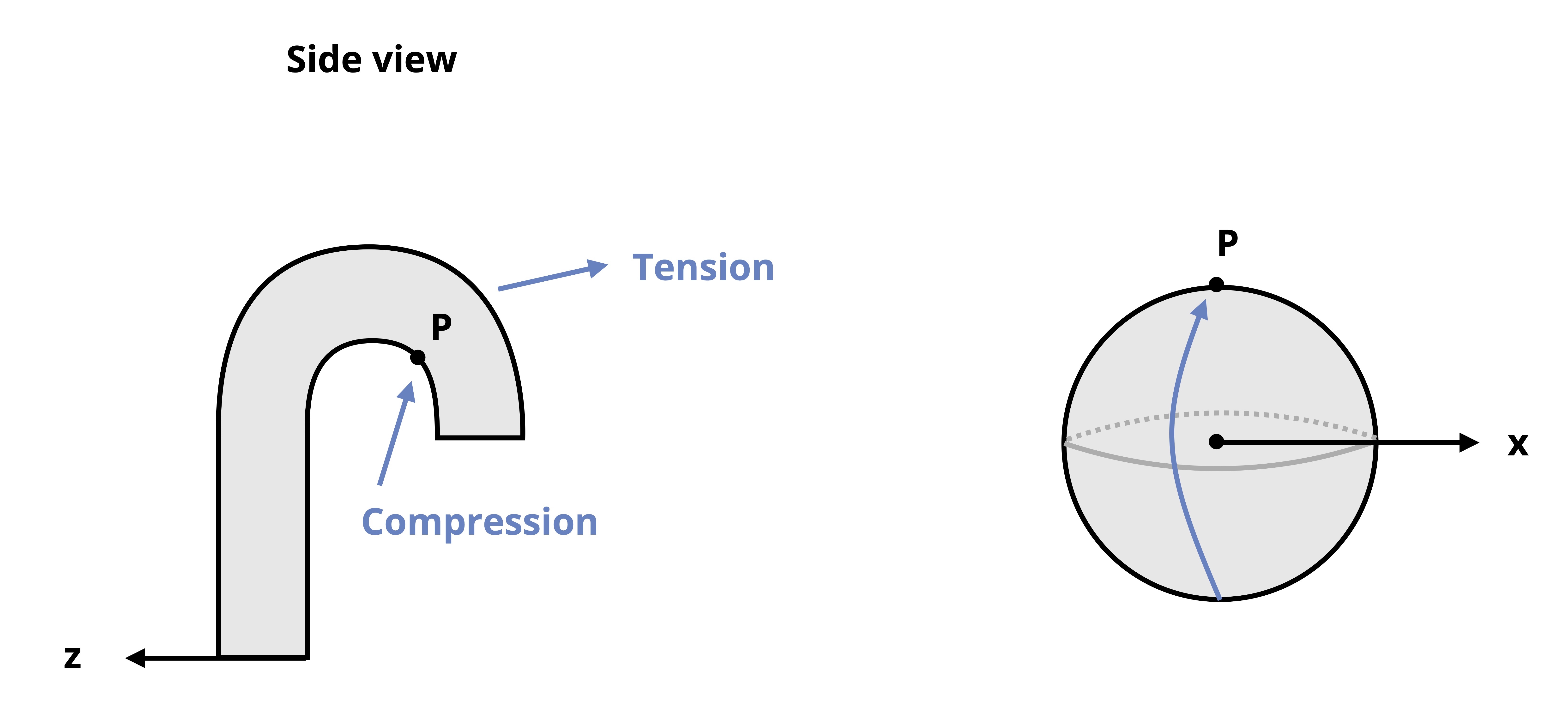
For point P, because it is on the centroidal z-axis, we know that it experiences no stress from Mz. Given the clockwise bending moment around the x-axis, the beam can be visualized as bending in a manner such that point P will be on the “inside” of the bend, or in compression.
If the visualization is difficult, we can also use the “tool” described in Section 14.1. Noting that the applied moment in this case is in the same direction as the bending moment (since equilibrium dictates that the moment at the fixed support is opposite of what is applied and the bending moment is opposite of the fixed support, we can conclude that the bending moment and applied moment would be in the same direction), we can draw the moment arrow across the cross-section. Note that this arrow should be drawn going over the x-axis. Drawing the arrow on the cross-section in this way, we can see that the arrowhead would point towards P, so all points above the x-axis, including P, are in compression from this moment.
The z distance from the x-axis to be P is the radius. We can then calculate the normal stress at point P to be:
\[ \sigma_{yP}=-\left|\frac{M_x z}{I_x}\right|=-\frac{376{~N}\cdot{m}*(0.016{~m})}{51.47 \times 10^{-9}{~m}^4}=-117{~MPa} \]
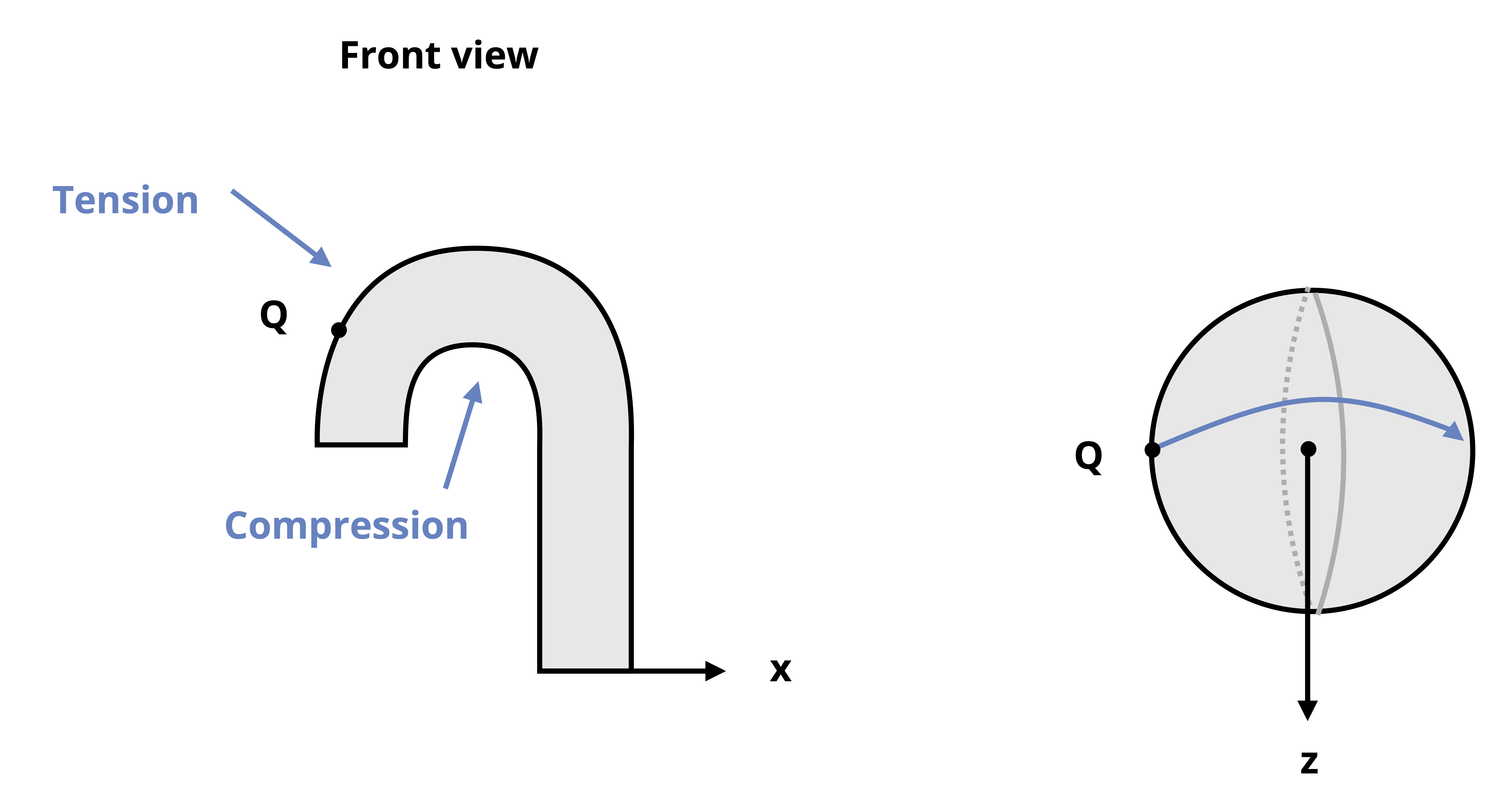
Similarly, point Q will experience no stress from Mx since it is on the x-axis, but it will feel stress from Mz. The x distance from the z-axis to point Q is also the radius. The sign on the stress can be determined by visualizing the bending to be as shown in the front view below and noting that point Q would be on the outside part of the bend. Alternatively, drawing the moment arrow on the cross-section as was done for point P above reveals that point Q is on the tail side of the arrow, so in tension.
The normal stress at point Q is thus calculated to be:
\[ \sigma_{y Q}=+\left|\frac{M_z x}{I_z}\right|=\frac{204{~N}\cdot{m}*(0.016{~mm})}{51.47 \times 10^{-9}{~m}^4}=63.4{~MPa} \]
σyP = 116.9 MPa (compression)
σyQ = 63.4 MPa (tension)
14.1.2 Eccentric Loading
When the line of action of an axial load does not pass through the centroid of a cross section, it will result in both a normal reaction force and a bending moment. For example, consider the traffic light and corresponding free body diagram shown in Figure 14.6.
The vertical support pole is subjected to normal forces from the weights of the traffic lights (the weight of the horizontal poles, cameras, etc., are assumed to be negligible for this example) as well as to bending moments around both cross-sectional axes (x and z) that result from the fact that the weights are not directly centered on the centroidal axes of the support pole. The total normal stress in the longitudinal direction, σy, at any given point on the pole would be given by the stress from the total normal force (\(\frac{\sum F_y}{A}\)) plus the bending stress from the bending moment around the z axis that results from W1 and W2 and the bending moment around the x axis that results from W3.
In terms of the general axes discussed in Section 14.1.1, we have:
\[ \boxed{\sigma_L= \pm\left|\frac{F_L}{A}\right| \pm\left|\frac{M_V d_H}{I_V}\right| \pm\left|\frac{M_H d_V}{I_H}\right|} \tag{14.2}\]
𝜎𝐿 = Bending stress in the longitudinal direction [Pa, psi]
FL = Internal normal force in the longitudinal direction [N, lb]
A = Cross-sectional area [m2, in.2]
MV = Bending moment around the vertical axis [N⸱m, lb⸱in.]
MH = Bending moment around the horizontal axis [N⸱m, lb⸱in.]
dH = Horizontal distance between the point on the cross-section for which the stress is being calculated and the V axis [m, in.]
dV = Vertical distance between the point on the cross-section for which the stress is being calculated and the H axis [m, in.]
IV = the moment of inertia about the vertical axis [m4, in.4]
IH = Area moment of inertia about the horizontal axis [m4, in.4]
The sign for the first term is positive if the total force is tensile (directed away from the cross-section) and negative if the total force is compressive (pointed towards the cross-section).
Example 14.2 and Example 14.3 demonstrate the calculation of normal stress in eccentric loading problems.
Example 14.4 goes through the process of calculating each of the components of normal stress and then combining them to determine the normal stress state at particular point.
Example 14.2
The structure is subjected to vertical forces as shown. Determine the total normal stress at points P and Q on the cross-section of the vertical portion of the structure.
The generalized normal stress equation is:
\[ \sigma_L= \pm\left|\frac{F_L}{A}\right| \pm\left|\frac{M_V d_H}{I_V}\right| \pm\left|\frac{M_H d_V}{I_H}\right| \]
In this case, the longitudinal axis (L) is the y-axis. The vertical axis of the cross-section (V) is the z-axis and the horizontal axis (H) is the x-axis.
To apply the equation, the internal reactions N, Mx, and Mz are needed. Since the internal reactions remain constant along the vertical portion of the structure, we can cut anywhere along its length to determine these internal reactions. The reaction moment around the x axis, Mx, can be determined to be 0 by inspection since all the forces pass through the centroidal x-axis of the cross-section. When finding the bending moments, it is important to remember that the moments needed are the moments around the centroidal axes of the cross-section.
\[ \begin{gathered} \sum F_y=N-75{~lb}-50{~lb}=0 \quad\rightarrow\quad N=125{~lb} \\ \sum M_z=(75{~lb}*15{~in.})-(50{~lb}*25{~in.})+M z=0 \quad\rightarrow\quad M z=125{~lb}\cdot{in.} \end{gathered} \]
Since both N and Mz are positive, the respective directions drawn on the FBD are confirmed to be correct. Thus, the normal force is compressive (pointed towards the cut section) and the bending moment is counterclockwise around the z-axis.
The total normal stress at point P can then be calculated with the following inputs:
\(F_L = N = 125{~lbs}\)
\(A = 6{~in.}*8{~in.} = 48{~in.^2}\)
\(M_V = M_x = 125{~lb}\cdot{in.}\)
\(d_x =\text{ x-distance between point P and the z-axis} = 2{~in.}\)
\(I_z = \frac{1}{12}*(6{~in.})*(8{~in.^3}) = 256{~in.^4}\)
The normal force N is compressive, so that term in the stress equation is made negative. With the counter-clockwise bending moment on the upper section, one can visualize that the bending would take on a “C” shape with point P on the outside of the bend, so point P would be in tension from the bending moment and that term in the equation is made positive.
As mentioned in Section 14.1.1, another way to determine the sign on the bending stress is to draw the direction of the overall applied moment on the cross-section. In this case, the total applied moment around the z-axis is:
\[ \begin{aligned} M=(75{~lb}*15{~in.})-(50{~lb}*25{~in.})&=-125{~lb}\cdot{in.} \\ &=125{~lb}\cdot{in.}~~\text{clockwise } \end{aligned} \]
Drawing the clockwise moment on the cross-section we see that the left side of the cross-section is on the tail side of the arrow, so we can conclude that all points to the left of the centroidal z-axis will be in tension. Note that for this tool to work, the arrow must always be drawn to be going “over” the axis as opposed to under.
\[ \sigma_{yP}=-\left|\frac{125{~lb}}{48{~in.^2}}\right|+\left|\frac{(125{~lb}\cdot{in.})(2{~in.})}{256{~in.^4}}\right| \\ \sigma_{yP}=-1.63{~psi} \]
The negative answer indicates that the stress is compressive.
To calculate the stress at point Q, all inputs to the equation remain the same except for dx. The x distance between the centroidal z-axis and point Q is 4 in. In addition, the sign on the bending stress is negative instead of positive since point K is on the inside of the bend (or on the arrow side of the cross-section drawn with the applied moment). Thus,
\[ \sigma_{yQ}=-\left|\frac{125{~lb}}{48{~in.^2}}\right|-\left|\frac{(125{~lb}\cdot{in.})(4{~in.})}{256{~in.^4}}\right| \\ \sigma_{yQ}=-4.56{~psi} \]
σyP = -3.49 psi, σyQ = -6.42 psi
Example 14.3
A force pulls up on point P on the post with rectangular cross section as shown. Determine the normal stress at point A.
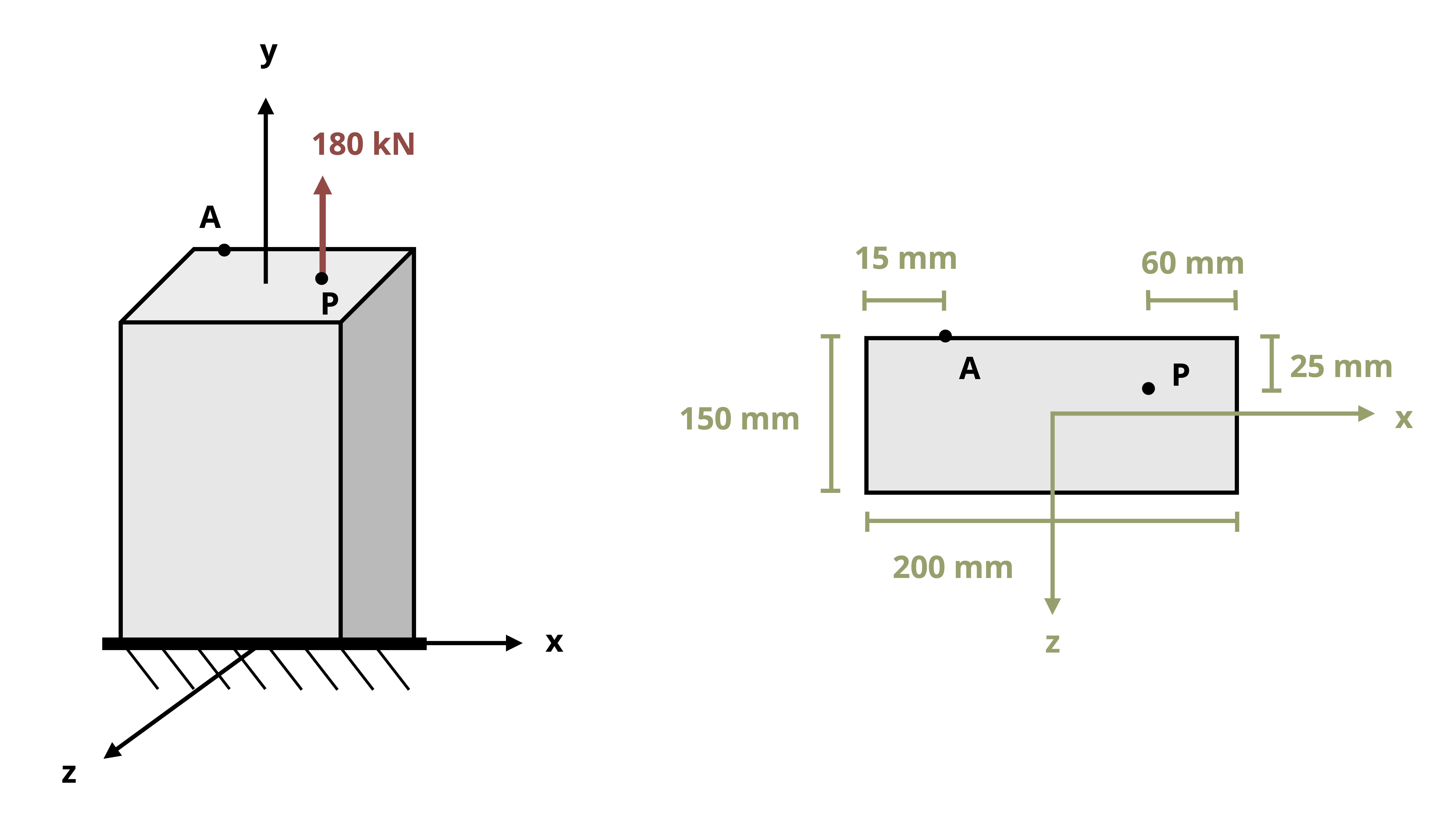
In this problem, there are three sources of normal stress: the bending stress from bending around the y axis, the bending stress from bending around the x axis, and the axial stress from the 180 kN force acting normal to the cross-section.
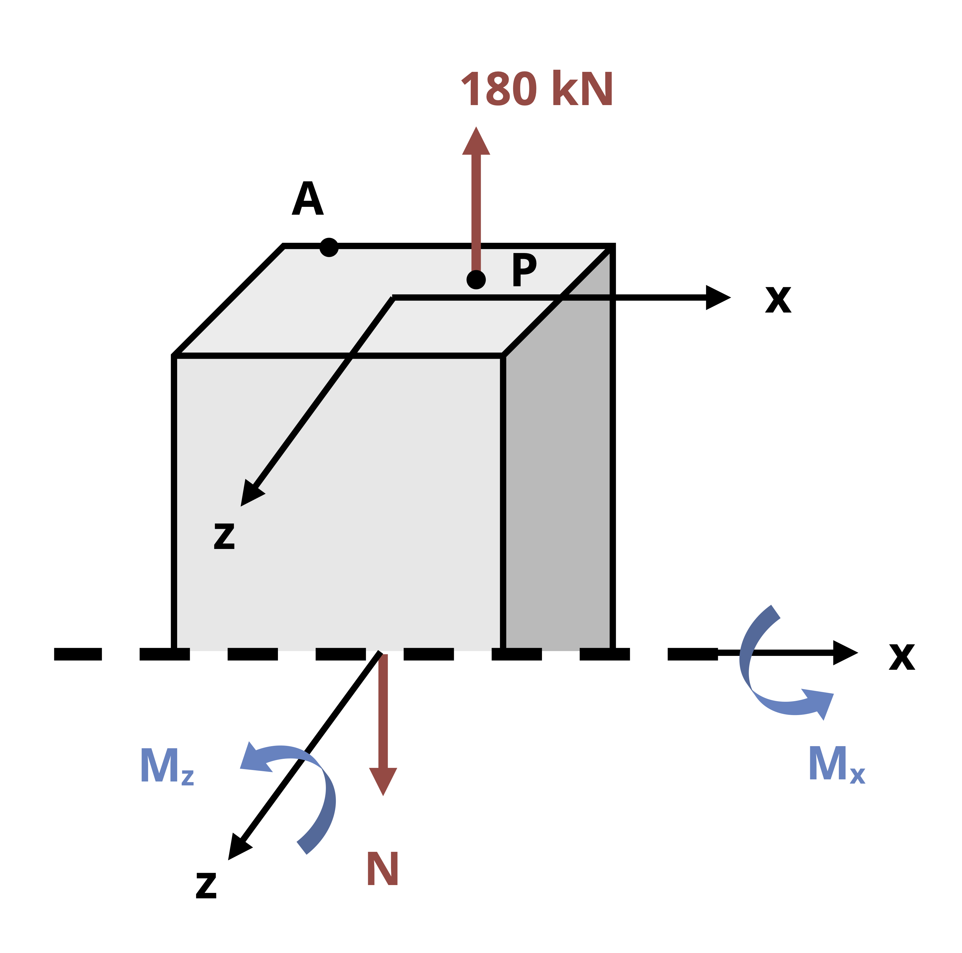
For the given loading, the internal reactions will be the same for any z location, so we can make a cut anywhere to determine the bending moment and normal force reaction
\[ \begin{aligned} &\sum M_X=(180{~kN}*50{~mm})+M_x=0 \quad\rightarrow\quad M_X=-9000{~kN}\cdot{mm} \\ &\sum M_Z=(180{~kN}*40{~mm})+M_z=0 \quad\rightarrow\quad M_Z=-7200{~kN}\cdot{mm} \\ &\sum F_Y=180{~kN}-N=0 \quad\rightarrow\quad N=180{~kN} \end{aligned} \]
By inspection of the applied moments, we can visualize that the bending around the x-axis is such that the post would bend towards us and points along the back edge where point A is would be in tension.
We can also visualize that the bending around the z-axis is such that the post would bend in a backwards C shape and points to the left of the centroidal z-axis would be in compression. We can also observe the the normal force reaction is tensile.
Applying the generalized normal stress equation (with the pressure term omitted):
\[ \sigma_{L A}= \pm\left|\frac{F_L}{A}\right| \pm\left|\frac{M_V d_H}{I_V}\right| \pm\left|\frac{M_H d_V}{I_H}\right| \]
In this case, the longitudinal axis of the post is the y-axis, the vertical axis of the cross-section is the y-axis, and the horizontal axis of the cross-section is x-axis. The dH in the equation is the x distance between centroidal z-axis and point A. The dV in the equation is the z distance between the centroidal x-axis and point A.
\[ \begin{aligned} &\sigma_{yA}=\left|\frac{N}{A}\right|-\left|\frac{M_z d_x}{I_z}\right|+\left|\frac{M_x d_z}{I_x}\right| \\ &\sigma_{yA}=\left|\frac{180,000{~N}}{(0.2{~m})(0.15{~m})}\right| \left|\frac{7200{~N}\cdot{m}*0.085{~m}}{\frac{1}{12}(0.15{~m})(0.2 {~m})^3}\right|+\left| \frac{9000{~N}\cdot{m}*0.075{~m})}{\frac{1}{12}(0.2{~m})(0.15{~m})^3}\right| \\ &\sigma_{y A}=11.9{~MPa} \end{aligned} \]
The stress works out to be positive and therefore tensile.
σyA =11.9 MPa
Example 14.4
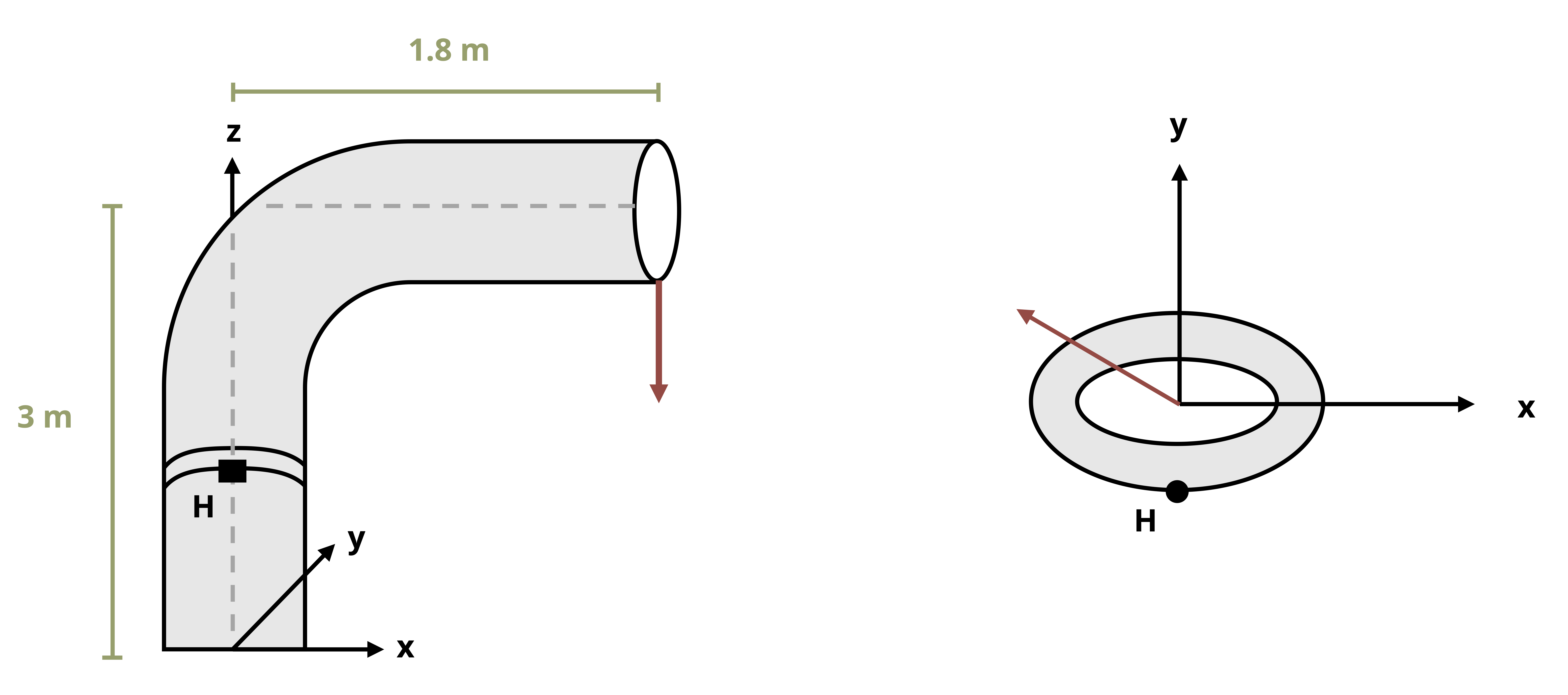
For the pressurized pipe loaded as shown, determine the normal stresses at point H. Noting that there would be no shear stress at point H for this loading, represent the general stress state of point H on a stress element. The pipe has an outside diameter of 200 mm and a wall thickness of 10 mm. The load Pz = 18 kN and the internal pressure in the pipe is 1500 kPa.
Consider the general normal stress equation:
\[ \sigma_L= \pm\left|\frac{F_L}{A}\right| \pm\left|\frac{M_V d_H}{I_V}\right| \pm\left|\frac{M_H d_V}{I_H}\right| \pm \frac{p r}{2 t} \]
In this problem, the longitudinal direction is the z direction and the horizontal and vertical axes of the cross-section where H is located are the x-axis and y-axis, respectively. Since there is pressure loading in this problem, there is also normal stress in the hoop direction (x and y-directions).
So we have:
\[ \begin{aligned} \sigma_{long} & = \pm\left|\frac{F_z}{A}\right| \pm\left|\frac{\left|M_y d_x\right|}{I_y}\right| \pm\left|\frac{\mid M_x d_y}{I_x}\right| \pm \frac{p r}{2 t} \\ \sigma_{hoop} & =\frac{p r}{t} \end{aligned} \]
Cutting through the part of the pipe where point H is located and applying equilibrium provides the following results for the internal reactions:
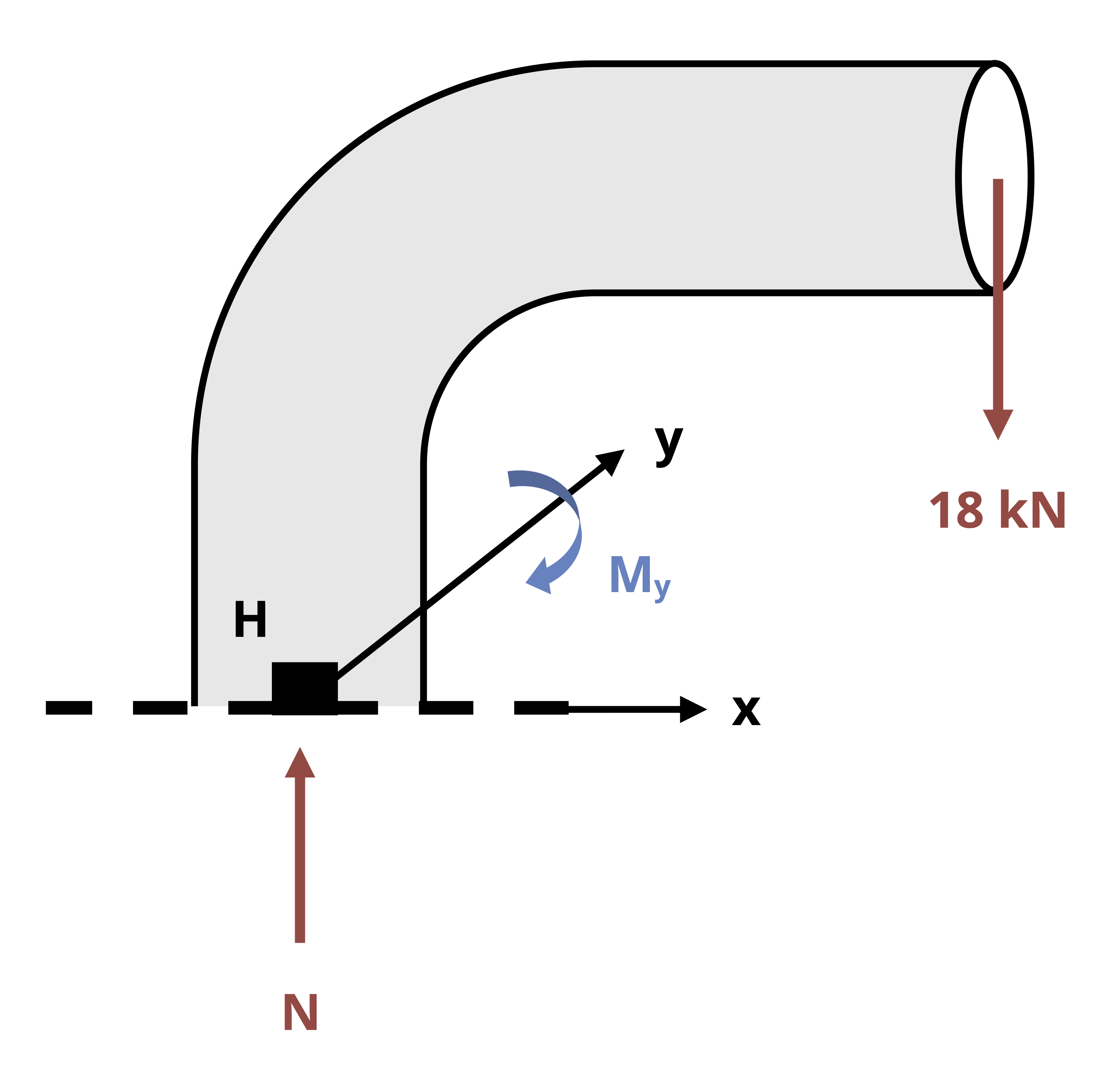
\[ \begin{aligned} &\sum F_y=N-18{~kN}=0 \quad\rightarrow\quad N=18{~kN} \\ &\sum M_y=(18{~kN}*1.8{~m})+M_y=0 \quad\rightarrow\quad M_y=-32.4{~kN}\cdot{m} \end{aligned} \]
Note that force is only applied in the z-direction so no other force reactions were drawn. There is also no force that results in a moment around the x-axis or z-axis, so Mx and Mz were also omitted from the FBD.
The normal force is positive based on the drawn direction, so it is compressive. The bending moment around the y-axis was drawn counterclockwise around the y axis, but the result is negative, so the bending moment is actually clockwise. However, since point H lies on the y-axis, there will be no stress at point H from this bending moment.
Thus the longitudinal stress (z-direction) becomes:
\[ \begin{aligned} \sigma_{long}&=-\left|\frac{F_L}{A}\right|+\frac{pr}{2t} \\ &=-\frac{18,000{~N}}{\pi\left(0.1^2-0.09^2\right){~m^2}}+\frac{(1,500,000{~Pa})(0.1{~m})}{2(0.01{~m})} \\ &=4.48{~MPa} \end{aligned} \]
The hoop stress (x-direction) is:
\[ \sigma_{hoop}=\frac{pr}{t}=\frac{(1,500,000{~Pa})(0.1{~m})}{0.01{~m}}=15{~MPa} \]
Now we can sketch a stress element at point H in the x-z plane.
14.2 General Shear Stress
Click to expand
Shear stress due to torsion was discussed in Chapter 6 while shear stress due to transverse loading was discussed in Chapter 10. In this section, the considerations that go into determining the total shear stress that arise when both forms of loading will be discussed.
14.2.1 Shear Stress due to Torsion
As discussed in Section 6.1, shear stress due to torsion can be calculated as:
\[ \tau_{(torsional)}=\frac{T \rho}{J} \]
For general problems, one may need to calculate T, so it is important to remember that torque is the moment about the longitudinal axis of a body, or that component of the moment that causes the body to twist. Since this form of shear stress will be combined with transverse shear stress to get the total, understanding the sign on the shear stress will be important.
Recall that when a stress element is drawn, a positive shear stress is one for which the shear stress arrow goes in the positive vertical direction on a positive vertical face and in the positive horizontal direction on a positive horizontal face. The positive or negative directions and faces are established by the positive sense of the axes which define the plane the point is in.
To determine which way a shear stress arrow would be drawn for a given stress element, one must cut the body at one edge of the stress element and visualize the direction in which the load would be applied across the cut.
For example, in Figure 14.7, when the cylinder is cut at the top of the stress element, we examine the bottom section of the cylinder and note that the reaction torque at the cut surface goes in the opposite direction to that which is applied at the bottom surface. This results in a counterclockwise reaction torque at the cut which means that the top section tends to want to twist (and exert a force) from left to right across the top element edge. If the vertical axis is positive upwards, the top face is a positive face. In addition, if the horizontal axis is positive to the right, the rightwards shear force arrow is in the positive direction. Together this means that the shear stress can be concluded to be positive since we would have a positive shear force on a positive face.
Similarly, when the cut is made at the bottom edge of the element, we can examine the top section of the cylinder for which equilibrium dictates that there is a clockwise reaction moment at the cut edge. This means that the bottom section tends to want twist from right to left across the bottom element edge. If the vertical axis is positive upwards so that the top face is a positive face, and the horizontal axis is positive to the right, the leftwards shear force would be a negative force acting on a negative face, so the shear stress would still be concluded to be positive.

14.2.2 Shear Stress due to Transverse Shear
In Chapter 10, the equation \(\tau=\frac{V Q}{I t}\) was evaluated to find the shear stress due to transverse shear force V. In that chapter, only one direction of shear force was considered for each problem and the sign on shear stress was not considered. For general loading, we may have two directions of transverse shear force corresponding to the two cross-sectional axes directions, as shown in Figure 14.8, so we will need to apply the transverse shear stress equation for both directions and also understand the signs so that we can combine them with each other and with the torsional shear stress.
When applying the transverse shear stress equations for specific directions of shear force, it is helpful to keep the following in mind:
- The cut one makes to determine the first moment of area Q will be perpendicular to the direction of shear force.
- The area moment of inertia will be the moment of inertia around the axis perpendicular to the shear force.
- The thickness, as before, refers to the thickness of the solid part of the cross section that one cuts through to calculate Q.
Using the same reference axes as with the general normal stress equation (H for horizontal centroidal axis and V for vertical centroidal axis), the transverse shear stress equation can be written as follows:
\[ \boxed{\tau_{(transverse)}= \pm\left|\frac{V_H Q_V}{I_V t_V}\right| \pm\left|\frac{V_V Q_H}{I_H t_H}\right|} \tag{14.3}\]
𝜏(transverse) = Transverse shear stress at point of interest [Pa, psi]
VH = Internal horizontal shear force [N, lb]
VV = Internal vertical shear force [N, lb]
QV = First moment of area about the vertical axis passing through the point of interest [m3, in.3]
QH = First moment of area about the horizontal axis passing through the point of interest [m3, in.3]
IV = Area moment of inertia about the vertical centroidal axis [m4, in.4]
IH = Area moment of inertia about the horizontal centroidal axis [m4, in.4]
tV = Vertical thickness of the cross-section [m, in.]
tH = Horizontal thickness of the cross-section [m, in.]
The signs on the shear stress are determined similarly to the manner described in Section 14.2.1 for torsion. The direction of the internal shear force is determined by equilibrium and this direction relative to the positive axes and faces on the stress element are used to establish direction.
It will be helpful to note that for any point on a cross-section that is on an edge that a transverse shear force goes through (or for a circular cross-section, any point on the outer diameter that lies in the path of the force), the transverse shear stress due to that direction of shear force is 0. This is illustrated in Figure 14.9. This is because the specified points would be on free surfaces in these cases. For example, for a vertical shear force, the bending would be around the horizontal axis, so the top and bottom surfaces would be considered free surfaces with no shear force acting above the top surface or below the bottom surface. The same would hold true for the left and right surfaces in the case of a horizontal shear forces that would result in bending around the vertical axis.
Example 14.5 demonstrates the calculation of transverse shear stress with multiple directions of shear force.
Example 14.5
Two forces are applied to a rectangular post as shown. Determine the shear stress at points P and S.
To find shear stresses at points P and Q, which are at the same vertical location on the post, we must first cut the post at that vertical location and find the internal reactions by applying equilibrium. The illustration below shows the section below the cut made at the cross-section where points P and Q are located. The reactions at the support due to the applied loading must be in the opposite direction to the loading for equilibrium and the internal reactions at the cut section will be opposite to the support reactions. Note that there are also bending moments around the x and y axes due to the applied forces, but those result in normal stress, not shear stress.
Given that there is no torsion in this problem, the general shear stress equation can be written:
\[ \tau= \pm\left|\frac{V_H Q_V}{I_V t_V}\right| \pm\left|\frac{V_V Q_H}{I_H t_H}\right| \]
Where the horizontal axis of the cross-section is the y–axis and the vertical axis of the cross section is the x-axis.
For any point on the cross-section, we can substitute:
\(V_H = V_y = 78{~kN}\)
\(V_V = V_x = 94{~kN}\)
\(I_H=I_y=\frac{1}{12}(160{~mm})^3(120{~mm})=40.96 \times 10^6{~mm}^4=40.96 \times 10^{-6}{~m}^4\)
\(I_V=I_x=\frac{1}{12}(120{~mm})^3(160{~mm})=23.04 \times10^6{~mm}^4=23.04 \times 10^{-6}{~m}^4\)
The Q and the t terms will depend on the specific points on the cross-section.
Point P:
The x faces of the post (front and back sides) do not feel shear stress from Vx since Vx results in bending around the y-axis and the front and back sides would be free surfaces for such bending. In the shear stress equation, we can also see this from that fact that Qy = A’x’ would be zero for point P (A’ = 0 below the horizontal cut at H and x’ = 0 for the area above the cut).
To find the shear stress from Vy, we would make a vertical cut through point H and calculate
\[ Q_x=A'y'=\frac{1}{2}(160{~mm})(120{~mm})*\left(\frac{1}{4}\right)(160{~mm})=384000{~mm}^3=384 \times 10^{-6}{~m}^3 \]
\(t_x = 120{~mm} = 0.12{~m}\)
Looking at the FBD of the cut section of the post drawn above, we can see that Vy goes across the top of the stress element of P in the positive y direction. The top of the element is on the positive z-face, so we a positive force on a positive face, which makes the resulting shear stress positive.
So
\[ \tau_P=\frac{V_y Q_x}{I_x t_x}=\frac{(78000{~N})(384 \times 10^{-6}{~m}^3)}{(40.96 \times 10^{-6}{~m}^4)(0.12{~m})}=6.09{~MPa} \]
Point S:
For point S, the shear stress from Vy will be zero by the same reasoning as used for point P and Vx (Qx = 0 for point S), so we only need to calculate the shear stress from Vx.
To find the shear stress from Vx, we would make a horizontal cut through point S and calculate
\[ Q y=A'x'=(160{~mm})(30{~mm})*(60{~mm}-15{~mm})=216000{~mm}^3=216 \times 10^{-6}{~m}^3 \]
\(t_y = 160{~mm} = 0.16{~m}\)
Again looking at the FBD of the cut post above, we can see that Vx goes across the top of the stress element for S in the negative x direction. So we a negative force on a positive face, which makes the resulting shear stress negative
So
\[ \tau_S=-\frac{V_x Q_y}{I_y t_y}=-\frac{(94000{~N})(216 \times 10^{-6}{~m}^3)}{(23.04 \times 10^{-6}{~m}^4)(0.16{~m})}=-5.51{~MPa} \]
τP = 6.09 MPa, τS = -5.51 MPa
14.2.3 Combined Shear Stress
Now we can consider the case of bodies having both torsion and transverse shear stresses. Given a general loading, one may need to calculate the torque and also identify which of the forces constitute transverse shear forces. It will be helpful to remember that the transverse shear forces are the forces in the directions of the cross-sectional axes and torsion is that component of moment that is about the longitudinal axis.
The total shear stress equation is:
\[ \boxed{\tau= \pm\left|\frac{T \rho}{J}\right| \pm\left|\frac{V_H Q_V}{I_V t_V}\right| \pm\left|\frac{V_V Q_H}{I_H t_H}\right|} \tag{14.4}\]
𝜏 = Shear stress at point of interest [Pa, psi]
T = Internal torque [N·m, lb·in.]
𝜌 = Radial distance from centroid to point of interest [m, in.]
J = Polar moment of inertia [m4, in.4]
VH = Internal horizontal shear force [N, lb]
VV = Internal vertical shear force [N, lb]
QV = First moment of area about the vertical axis passing through the point of interest [m3, in.3]
QH = First moment of area about the horizontal axis passing through the point of interest [m3, in.3]
IV = Area moment of inertia about the vertical centroidal axis [m4, in.4]
IH = Area moment of inertia about the horizontal centroidal axis [m4, in.4]
tV = Vertical thickness of the cross-section [m, in.]
tH = Horizontal thickness of the cross-section [m, in.]
Example 14.6 demonstrates the calculation of total shear stress when torsion and transverse shear are both acting.
Example 14.6
A solid steel bar with an outside diameter of 6.70 in. is loaded as shown. Determine the maximum shear stress at points J and K on the outside of the pipe.
First we need to find the internal reactions at the location of the points in question. To find the internal reactions, we will first draw the whole body FBD and apply equilibrium to find the reactions at the support. Then we will cut the body at the location of points J,K and apply equilibrium to the cut section to find the internal reactions. All the reactions are calculated below even though we only need Vx, Vz, and My to find the shear stresses.
To find reactions at support:
\[ \begin{aligned} & \sum F_x=R_x+1500{lb}=0 \quad\rightarrow\quad R_x=-1500{~lb} \\ & \sum F_y=R_y=0 \\ & \sum F_z=R_z+900{~lb}=0 \quad\rightarrow\quad R_z=-900{~lb} \end{aligned} \]
\[ \begin{aligned} & \sum M_x=M_{Rx}+(900{~lb})(80{~in.})=0 \quad\rightarrow\quad M_{Rx}=-72,000{~lb}\cdot{in.} \\ & \sum M_y=M_{Ry}+(900{~lb})(18{~in.})=0 \quad\rightarrow\quad M_{Ry}=-16,200{~lb}\cdot{in.} \\ & \sum M_z=M_{Rz}-(1500{~lb})(80{~in.})=0 \quad\rightarrow\quad {Mz}=120,000{~lb}\cdot{in.} \end{aligned} \]
To find reactions at cut section:
\[ \begin{aligned} & \sum F_x=R_x+V_x=-1500{~lb}+V x=0 \quad\rightarrow\quad V x=1500{~lb} \\ & \sum F_y=R_y+V_y=0 \quad\rightarrow\quad V y=0 \\ & \sum F_z=R_z+V_z=-900{~lb}+V_z=0 \quad\rightarrow\quad V_z=900{~lb} \end{aligned} \]
\[ \begin{aligned} & \sum M_x=M_{Rx}+V_z(10{~in.})+M_x=-72,000{~lb}\cdot{in.}+900{~lb}(10{~in.})+M_x=0 \quad\rightarrow\quad M_x=63,000{~lb}\cdot{in.} \\ & \sum M_y=M_{Ry}+M_y=-16,200{~lb}\cdot{in}+M_y=0 \quad\rightarrow\quad M_y=16,200{~lb}\cdot{in.} \\ & \sum M_z=M_{Rz}-V_x(10{~in.})+M_z=120,000{~lb}\cdot{in.}-1500{~lb}(10{~in.})+M_z=0 \quad\rightarrow\quad M_z=-105,000{~lb}\cdot{in.} \end{aligned} \]
The longitudinal direction based on the part of the rod on the y-axis is the y-axis, so the torsional moment is My. Both points J and K will experience the same magnitude of shear stress from the torsion, however, it is possible for the signs to be different for the two different points depending on orientation. The magnitude of the shear stress is:
\[ \tau_{torsion}= \pm\left|\frac{Tc}{J}\right|=\pm\left|\frac{M_y(c)}{J}\right|= \pm\left|\frac{16,200{~lb}\cdot{in.}*(3.35{~in.})}{\frac{\pi}{32}(6.7{~in.})^4}\right|= \pm 274{~psi} \]
Considering the stress element for each point with the counterclockwise torque resulting in a downwards directed force across the cut face of the element, we can note that there would be a negative z force on a positive y face for point K and a positive x force on a positive y face for point J. So
\(τ_{K(torsion)} = - 274{~psi}~~\text and~~ τ_{J(torsion)} = + 274{~psi}\)
Now turning our attention to the shear stresses from the transverse forces, we note the cross sectional axes are the x- and z-axes, so the transverse shear forces are those that are in the x- and z-directions. We can also note that with K being on the x-axis of the cross section, it will not experience transverse shear stress from Vx. Similarly, point J will not experience transverse shears tress from Vy. In addition, since the cross-section is circular, we know that for both points:
\[ \begin{aligned} & Q_{max}=\frac{1}{12} d^3=\frac{1}{12}(6.7{~in.})^3=25.06{~in.^3} \\ & t=d=6.7{~in.}^3 \\ & I_x=I_z=\frac{\pi}{64} d^4=\frac{\pi}{64}(6.7{in.})^4=98.92{~in.^4} \\ & \end{aligned} \]
Since Vz acts in the positive z direction on the positive y face for point K, the transverse shear stress for point K is positive. Since Vx acts in the positive x direction on the y face for point Y, the transverse shear stress for point J is also positive.
\[ \begin{aligned} & \tau_{K(transverse)}= \pm\left|\frac{V_z Q_{circle}}{I_{circle} d}\right|=+\frac{900{~lb}(25.06{~in.}^3)}{98.92{~in.}^4(6.7 {~in})}=34.03{~psi} \\ & \tau_{J(transverse)}= \pm\left|\frac{V_x Q_{circle}}{I_{circle} d}\right|=+\frac{1500{~lb}(25.06{~in.}^3)}{98.92{~in.}^4(6.7 {~in.})}=56.72{~psi} \end{aligned} \]
Finally, we can calculate the total shear stress for each point by summing the torsional shear stress with the transverse shear stress:
\[ \begin{aligned} & \tau_K=\tau_{(torsion)}+\tau_{(tranverse)}=-274.3{~psi}+34.03{~psi}=-240.27{~psi} \\ & \tau_J=\tau_{(torsion)}+\tau_{(tranverse)}=274.3{~psi}+56.72{~psi}=331.02{~psi} \end{aligned} \]
τK = -240.27 psi, τJ = 331.02 psi
14.3 General Combined Stress
Click to expand
Once the total normal stress and total shear stress at a specified point is calculated, the general stress state can be represented on a stress element and used to determine principal stresses, principal planes, and max/min shear stresses.
In Example 14.7, the problem from Example 14.5 is extended to find the principal stresses and max/min shear stresses.
Example 14.7
Revisit Example 14.5 to find the principal stresses and max/min shear stresses for point P on the post:
In Example 14.5 the total shear stress for point P was found to be positive 6.094 MPa.
To find the principal stresses, we must finish finding the general stress state by also finding the normal stresses and then use the principal stress equations or Mohr’s Circle.
The normal stress for this problem only arises from the bending around the x- and y-axes (the cross-sectional axes) since there is no force in the longitudinal z-direction and there is no pressure involved. The bending stress will be in the z-direction since that is the longitudinal direction.
In addition, since P is on the x-axis, it will experience no stress from the moment around the x-axis, Mx, so all the normal stress comes from the bending around the y axis, My.
As discussed in Example 14.5, if we consider the FBD of the section cut at P shown below, we know by inspection that the internal reactions at P will be the same magnitude and direction as the applied. This is because the reactions at the support will be equal and opposite to the applied and the internal reactions are the opposite of those.
The internal moment reaction around the y-axis, My, can then be calculated as:
\[ \begin{aligned} \sum M_y=(-94{~kN})(150{~mm})&=-14,100{~kN}\cdot{mm} \\ &=14,100{~kN}\cdot{mm}~~\text{clockwise} \end{aligned} \]
The bending stress for point P will be positive since the clockwise moment around the y-axis means that the post will curve into the plane of the screen and look as shown below from the positive y side view. The cross-section is also shown with the tail of the representative moment arrow on the P side of the cross-section, indicating that everything below the y-axis will be in tension.
Recalling \(I_y = 40.96 \times 10^{-6}{~m^4}\) from Example 14.5, the normal stress at P is then:
\[ \sigma_{P z}=\frac{M_y x}{I_y}=\frac{14,100{~N}\cdot{m}(0.06{~m})}{40.96 \times 10^{-6}{~m^4}}=20.7{~MPa} \]
Now that the total shear stress and total normal stress are known, the stress state can be represented on a stress element.
Applying the simplified version of the principal stress equations and the max/min shear equation (in terms of the general xy plane), we get:
\[ \begin{aligned} & \sigma_{1,2}=\frac{\sigma_x+\sigma_y}{2} \pm \sqrt{\left(\frac{\sigma_x-\sigma_y}{2}\right)^2+\tau_{x y}{ }^2} \\ & \tau_{\max , \min }= \pm \sqrt{\left(\frac{\sigma_x-\sigma_y}{2}\right)^2+\tau_{x y}{ }^2} \end{aligned} \]
In this case, since the point P is in the y-z plane instead of the x-y plane, we can replace the x subscripts with y and the y subscripts with z, so the equations become:
\[ \begin{aligned} & \sigma_{1,2}=\frac{\sigma_y+\sigma_z}{2} \pm \sqrt{\left(\frac{\sigma_y-\sigma_z}{2}\right)^2+\tau_{y z}^2}=\frac{20.7{~MPa}+0}{2} \pm \sqrt{\left(\frac{20.7{~MPa}-0}{2}\right)^2+(6.094{~MPa})^2}=22.26{~MPa},-1.661{~MPa} \\ & \tau_{\max , \min }= \pm \sqrt{\left(\frac{\sigma_y-\sigma_z}{2}\right)^2+\tau_{y z}^2}=\sqrt{\left(\frac{20.7{~MPa}-0}{2}\right)^2+(6.094{~MPa})^2}=12.01{~MPa},-12.01{~MPa} \end{aligned} \]
σ1 = 22.36 MPa
σ2 = 22.36 MPa
τmin = -12.01 MPa
τmax = 12.01 MPa